
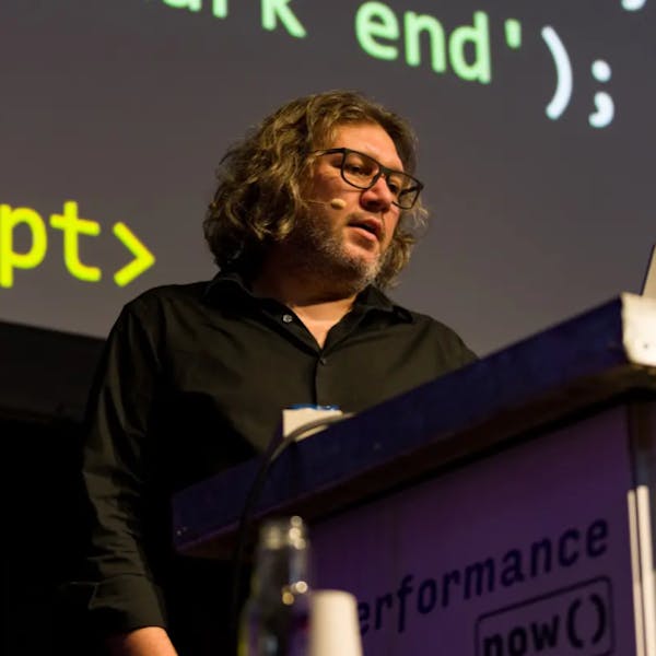
Stoyan (@stoyan.org) is currently consulting for Etsy, Previously of Webpagetest.org, Facebook and Yahoo, writer ("JavaScript Patterns", "React: Up and Running"), speaker (dotJS, JSNation, Performance.now()), toolmaker (Smush.it, YSlow 2.0) and a guitar hero wannabe.
Remember YSlow? If you do, skip to the next header.
YSlow?
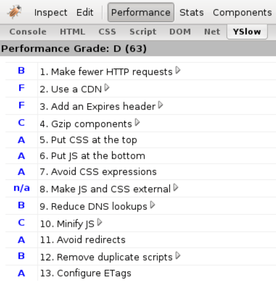
Back in the olden days circa 2007-ish, there appeared a tool called YSlow. It was a Firefox extension (Chrome wasn’t a thing, not even a sparkle in anyone’s eye) that codified 13 best practices for speeding up web pages based on research by Steve Souders and other assorted Yahoo! folks. Yahoo! was/is an array of web sites, some dedicated to TV, some to music, gossip, finance, etc. And developers working on these diverse sites shared their experience with the world in the form of these 13 best practices, aka “rules” that were even graded by YSlow using the US system where A is the best, B is a little less than perfect and so on.
The 13 “rules” became 14, then 34… At this point we needed to categorize and in a way revert to a pre-YSlow world where web perf is not really that simple and a dozen rules won’t do.
But this was the amazing feat of YSlow… actually let me quote Eric Lawrence:
“Steve Souders has done a fantastic job of distilling a massive, semi-arcane art down to a set of concise, actionable, pragmatic engineering steps that will change the world of web performance.”
Years later, Google followed suit with PageSpeed, another Firefox extension which later morphed into other things and eventually there came Lighthouse, which is still around.
My involvement? I was responsible for YSlow 2.0 after Steve left Yahoo! which brought the 14 rules to 34 and introduced extensibility, categories, custom rules (e.g. SEO) etc. Lighthouse-y stuff.
Fast forward to last month, I was invited to an “AI & performance” summit and decided to revive the old YSlow idea into today’s world and see if we can have AI discover and codify, nay distill, a bunch of data into a set of best practices (or rules) that somewhat match the original 13 that came with YSlow. Hence aiSlow…
AI web performance consultant
YSlow (pronounced “Why Slow?”) meets aiSlow (pronounced “Eh, I Slow?”).
First we need to train the consultant model. How do we go about that? Well, we need data.
Naïve take
My first impulse was to have an AI of sorts ™ take a bunch of HARs and spit out wisdom! Turns out that unguided “deep learning” based on raw messy JSON data is not for the faint of heart. We need something more structured, like an Excel sheet.
In that “Excel” sheet we need to differentiate a Target vs Features. The target is a good desired outcome. The features are pieces of data hopefully related to the target.
So what’s every AI model’s first task?
Crawl the web and collect!
Yup, crawl aggressively, borderline abusively poor unsuspecting sites to get that juicy, juicy data.
Nah, HTTPArchive
On second thought… we already have HTTPArchive.org which crawls millions of pages monthly and saves the crawl data in BigQuery.
So we’re skipping the crawl and getting some data that is already crawled.
But what type of data to get?
Naïve take
Let’s just pick 10K random URL and learn!
Turns out this is not the best of ideas, the data is all over the place.
The slows and the fasts
A much better approach is to take a bunch of slow pages and a bunch of fast pages and learn from these. Also a good idea is to filter out pages that are too fast (error pages, forbidden, N/A in your country) or too slow (temporary issues, timeouts).
The HTTPArchive also has the concept of page rank (popularity). We’ll err on the side of the more popular pages, presuming these are developed by more dedicated teams who know what they’re doing.
But we want 10K fast pages and 10K slow ones and if we cannot get enough data from the highest ranking pages, we’ll fill up with a random selection of lower ranked ones.
Target & Features
Features
The features are about 60-ish pieces of data that seemed relevant to web performance: TTFB (Time to first byte), caching headers and so on.
Target
That was the age-old question: what single metric (it needs to be one for the AI training) defines what a fast page is.
My initial thought was to define an aggregate of some sort like take TTFB, add DOMContentLoaded time, add onload time (multiplied by 0.5 because it’s not that important), add Largest Contentful Paint (multiplied by 1.5 because it’s more important) and so on….
But then.. what about SpeedIndex? A wonderful metric that combines all of CWV and more into a single number. Perfect! This is the target.
Query
Here’s an example query used to get HTTPArchive data and these are the CSV results: fast 5000, more 6000 fast ones, 13K slow ones.
Learning
Now we dive into AI territory which may be as new to the reader of this publication as it was to me.
We’ve all seen LLMs (like ChatGPT) but this is not our goal. We don’t need prose generated.
There’s also “deep learning” – given a bunch of nonsense data, try to get some wisdom. But this is not our task either. This is more for unstructured data like images and video. A bunch of HARs may be close but they are not so unstructured, as messy as they are, they are still pages and request info.
Now we’re down to the easy types of learning/training: Regression (predicting a number) vs. Categorization (is this a cat or a dog?).
We are definitely not categorizing.
We’re not predicting either. The goal of the tool, as the goal of the original YSlow, is to take the results for a web page (including SpeedIndex, our target) and tell us why it’s slow/fast and what can we do to make it faster.
Yet prediction is the type of training most suitable for our goal. Our trained model will predict the SpeedIndex (SI) and we can see how good the prediction is is by comparing the predicted SI with the real one. But that’s just for our use, to judge the quality of the model. The real output is still going to be: what can we do to make the page faster, based on the knowledge of all these other pages we use for training.
At this point you may realize that some of the concepts match what Ethan Gardner described in his Calendar post, so do check this one as well for a better understanding.
LightGBM: Light Gradient Boosting Machine
Now we’re getting deeper into AI weeds. We’ve settled on using a regression algorithm. One such algo and framework is LightGBM, a “gradient-boosting” framework developed by Microsoft that uses tree-based learning algorithms. It can do both regression (LGBMRegressor) and categorization (dog vs cat).
LGBMRegressor is the specific model “class” we’ll use.
LightGBM
This framework will take our structured CSV data with web performance metrics (bytes, number of requests, etc.) and train a regression model to predict SpeedIndex (SI).
It uses decision trees to find patterns in the data. The underlying idea is fairly straightforward. The algorithm makes a bold (and almost certainly wrong) prediction, like “pages with 7 requests are slow (SI is 9000ms)”. It splits the data into pages with less than and more than 7 requests. And sees how wrong it is.
Then it goes back and tries to correct the splitting. And so it assembles decision trees, each one correcting the previous one.
In general for a case like this around 500 corrections of previously wrong splits of data should yield a good outcome.
Let’s go!
As many (all?) programs, we have the sequence of input-magic-output.
Input
- Desktop-only HTTPArchive data
- Target: SpeedIndex
- Features: 60-ish pieces of data for each page
- 11000 fast pages (fast is defined as having SI between 500 and 2500ms)
- 13000 slow pages (SI is between 4500 and 20000ms)
Magic
Our script is a Python file called train_model.py. In it you can see some hardcoded numbers that need explaining:
- 80/20 train/test split (
test_size=0.2). This is a common good practice, use 80% of the data for training and check against the other 20% if the training makes sense. Otherwise the model just rote-learns some values (overfitting). - Categorical Features: some features are just continuous numbers like SpeedIndex 564 or 4789. Others are boolean (uses CDN: yes/no) or just few enough distinct values, say render-blocking CSS files. More “categories” (not too many distinct values) is better. You can see the chosen features to be categories here.
DataFrame– this is a data format preferred by the algorithm. Think of it as better CSV.random_state=42. The42value can be anything. Any value means reproducible results, easier to debug, because the necessary randomness of the algorithm (where to split) is fixed to the same randomness every time.n_estimators=500– This is the maximum number of “boosting rounds” or corrections of the previous wrong splits.learning_rate=0.05means more careful, gradual learning. A prediction is Tree1 + 0.05 * Tree2 + 0.05 * Tree3 + …stopping_rounds=10. This is so we can exit before the 500 rounds. If 10 consecutive corrections don’t improve anything, call it done.
Output
The Trained Model, aka The Brain, is the output of the script. It takes the form of a file called aislow_desktop.pkl. PKL = PICKLE. This is a Python-preferred file format that is human readable and not too far from a simple serialized dump of an object from memory. Here it is.
Running the training script
Here’s the exact console printout of running the training script:
$ python3 train_model.py
Starting model training process...
Loading and combining 3 CSV files...
  Loading 'fast 6k - rank under 10k si 500 to 2500.csv'...
    Loaded 6089 rows
  Loading 'fast 5k - rank under 50k si 500 to 2500.csv'...
    Loaded 5000 rows
  Loading 'slow 13k - rank under 100K si 4500 to 20k.csv'...
    Loaded 13347 rows

Combining all datasets...
Successfully combined into 24436 total rows and 65 columns.
Checking for duplicate URLs...
  Removed 1640 duplicate URLs
Checking for missing values in 'SpeedIndex'...
  No missing values in target column
Separating features (X) and target 'SpeedIndex' (y)...
Dropping 'page' (URL) and target 'SpeedIndex' from features...
Excluding 4 additional feature(s): FirstMeaningfulPaint, FirstImagePaint, FirstContentfulPaint, LargestContentfulPaint
Converting specified columns to 'category' type...
  Converted: ['uses_cdn', 'reqCss', 'reqFont', 'reqJS', 'renderBlockingCSS', 'renderBlockingJS', 'num_long_tasks', 'analytics', 'ads', 'marketing', 'fonts_scripts', 'tagman', 'chat', '_responses_404', 'is_lcp_preloaded', 'scripts_defer', 'scripts_async', 'scripts_inline']

Features (X) shape: (22796, 59)
Target (y) shape: (22796,)
Splitting data into training and test sets (80% train / 20% test)...
Initializing LGBMRegressor model...
Starting model training... (This should be fast!)

--- Training Complete ---
Training took 1.26 seconds.
Best iteration: 111
Model R-squared score on test data: 0.5754

Top 13 Most Important Features:
Feature                                  Splits   Gain %    Correlation  Impact
-----------------------------------------------------------------------------------------------
Total Page Size (Bytes)                  201      44.84     0.355        ↑↑ SLOWS page
First Paint                              354      23.92     0.511        ↑↑ SLOWS page
JavaScript Requests (Count)              360      4.28      0.367        ↑↑ SLOWS page
Time To First Byte (ms)                  162      3.51      0.339        ↑↑ SLOWS page
JavaScript Size (Bytes)                  117      2.27      0.486        ↑↑ SLOWS page
Async Scripts                            222      2.27      0.249        ↑ slows page
Long Tasks Count                         154      1.94      0.368        ↑↑ SLOWS page
Inline Scripts                           185      1.92      0.171        ↑ slows page
Image Size (Bytes)                       105      1.28      0.288        ↑ slows page
Total Blocking Time                      101      1.14      0.348        ↑↑ SLOWS page
Max Requests Per Domain (Count)          51       0.95      0.327        ↑↑ SLOWS page
CSS Requests (Count)                     102      0.87      0.246        ↑ slows page
Total Scripts                            32       0.58      0.307        ↑↑ SLOWS page

Note: Correlation shows LINEAR relationship with SpeedIndex.
      Positive = higher values → higher SpeedIndex (slower)
      Negative = higher values → lower SpeedIndex (faster)
      The model may capture more complex non-linear patterns.

Saving trained model to 'aislow_desktop.pkl'...
---
Success! Trained model saved.
Understanding the output
After running train_model.py, we get some interesting numbers to look at:
Training took 1.26 seconds
Yup, just over a second. This is one of the good things about LightGBM – it’s fast. Remember we’re processing 24,000 pages with ~60 features each. Deep learning would’ve taken hours and require a GPU.
Best iteration: 111
Remember we set n_estimators=500 (maximum 500 rounds) and stopping_rounds=10 (quit if 10 consecutive rounds don’t improve)? Well, the model figured out the patterns after just 111 rounds of corrections. After that, it continued wheel-spinning for 10 more attempts, noticed the lack of improvements and threw them away stopping at the 111th attempt.
This tells us our model converged relatively quickly. The data isn’t so messy that it needs all 500 attempts to figure things out.
Model R-squared score on test data: 0.5754
This is the moment of truth. R-squared measures how well our model predicts the test data. It ranges from 0 to 1:
- 1.0 = Perfect predictions, it never happens unless we’re overfitting (just memorizing all the data). Close to 1 is preferable for categorization (is it a cat or a dog?) but not regression.
- 0.5754 = We’re explaining about 58% of the variance in SpeedIndex
- 0.0 = The model is useless, might as well predict the average every time
So is 0.5754 good? For web performance, yes. Remember, web pages are messy and unpredictable. Networks vary, servers have bad days, third-party scripts are just plain weird. Getting 58% accuracy on predicting something as complex as SI from just 60 features is actually pretty impressive.
More importantly, we’re not building a crystal ball. We don’t need perfect predictions. We need to understand which features matter most – and for that, this model is more than adequate.
Feature importance
The training script spits out a table showing which of the ~60 features matter most for predicting SI. For each feature, we get three metrics:
Splits – How many times the feature was used across all decision trees. If bytesJS appears in 1000 tree splits, it means the model kept asking “Is JavaScript size more or less than X?” throughout its learning. High splits means the feature is used frequently, but doesn’t tell us if it actually matters or just helps making tiny adjustments.
Gain % – The percentage of total prediction improvement attributed to this feature. This is the most important metric. If a feature has 25% gain, it means a quarter of the model’s predictive power comes from this one feature. This is what we want to focus on when understanding what drives performance.
Correlation – The linear relationship between the feature and SI, ranging from -1 to +1. Positive means “more of this slows pages down”, negative means “more of this speeds things up”. But here’s the catch – correlation only captures linear relationships. The model can see complex non-linear patterns that correlation misses. For example, TotalBlockingTime might have low correlation if the relationship is something like “100ms or less is fine, but 100-1000ms is a performance slayer”.
The hierarchy is: Gain >> Splits > Correlation
When interpreting results, we look at Gain % first – it tells us what the model actually relies on. Splits shows frequency of use. Correlation is useful as a sanity check for direction (does more JavaScript slow things down? yes, good) but don’t overweight it since the model sees patterns beyond simple linear relationships.
In practice with the data available to us in HTTPArchive, more of anything is bad for performance (every byte is precious) or neutral. Except for the use of CDN where more (well true vs false) is better.
Will it replicate YSlow’s original 13?
If you look back at the training script output, in the “Top 13 Most Important Features” was my attempt to match the original YSlow 13. As you can see, other than number of requests of various types, little else matches.
But that’s ok. One big limitation of the training data is that we didn’t use data about the contents of the requests, so for example we can’t see if the CSS is at the top and JS at the bottom.
Some data like the Expires headers we do have, but it’s not really relevant to the SI, it’s more for the consecutive page views.
All in all looks like the training concluded with ideas like more = bad for performance. No kidding, right?
Let’s move on. Now that we have a trained model we can unleash it on new pages that are not in the training set. I just pick a random page from a new set of a 100 test pages, also selected from the HTTPArchive.
aislow.py
This is the actual “webperf consultant in a box”, source.
We give it a page (from a test set, not in the training data) and it tells us what’s slowing it down and what can be improved. This is the whole point of the exercise – replicating what YSlow did with its graded rules, but now driven by data and machine learning.
The script needs three things:
- The trained model (
aislow_desktop.pkl) - The page data we want to analyze (from a CSV)
- The training data (for context and baseline calculations). This one took me by surprise, why would you need the raw data every time, and turns out a representative sample can be good enough. It’s only for figuring out percentiles across the whole data set.
The script loads the model, picks a page, runs it through the model to get a prediction, then uses SHAP (SHapley Additive exPlanations) to break down the prediction into individual feature contributions.
SHAP is the key here. It’s a technique from game theory that answers: “How much did each player (feature) contribute to the final outcome (prediction) of a game?” (Think a football game). For each feature, SHAP calculates its impact in actual milliseconds – not just “this matters” but “this adds +450ms to your SI”.
The output is a text report showing:
- The page URL
- Actual vs predicted SI
- Top 5 problems (features adding 50ms+, anything under is likely just noise)
- Top 3 strengths (features saving 50ms+)
- A “what-if” scenario (what happens if we fix the #1 problem?)
Plus a SHAP waterfall plot saved as a PNG showing the visual breakdown.
Here’s a real example from running the script:
python3 aislow.py
Training data: 24436 pages
  Average SpeedIndex: 5519 ms
  Median SpeedIndex: 5114 ms

---------------------------------------
---------     EH, I SLOW?     ---------
---------------------------------------
Page: https://urban96.fm/
SpeedIndex: 1761ms (actual)
Predicted SpeedIndex: 1601ms
Prediction error: 160ms

--- Top Problems (Areas for Improvement) ---
No significant problems found.

--- Top Strengths (What's Working Well) ---
  * Total Page Size (Bytes) = 2,159,952
    └─ Impact: -1344 ms
  * First Paint = 920
    └─ Impact: -1165 ms
  * JavaScript Size (Bytes) = 166,128
    └─ Impact: -430 ms

--- What-If Simulation ---
No problems to simulate.
In this case the page is fast, faster than the median SI in the training data (5114ms). And there’s even nothing to improve. Funny that 2MB of page is a strength, because that’s way under the median. Being so light (comparatively) gives it an estimated boost of 1344ms
What-If
Did you notice the what-if part? For this feature we take the top #1 worst offending feature, pretend it’s in the 25th percentile (change its value to a good desired one) and recalculate the prediction. The goal is to see what will happen to SI if we improve that worst offender by this much.
This is neat and very AI-ish. YSlow didn’t tell us how much faster a page will be if we move a score for example from D to B.
Let’s take a look at an example that does have the what-if:
python3 aislow.py
Training data: 24436 pages
  Average SpeedIndex: 5519 ms
  Median SpeedIndex: 5114 ms


---------------------------------------
---------     EH, I SLOW?     ---------
---------------------------------------
Page: https://muscomm.ru/tpost/anob2oorb1-kak-razvit-muzikalnii-sluh-vzroslomu-upr
SpeedIndex: 4807ms (actual)
Predicted SpeedIndex: 5695ms
Prediction error: 888ms

--- Top Problems (Areas for Improvement) ---
  * First Paint = 3,648
    └─ Impact: +1165 ms
  * Async Scripts = 32
    └─ Impact: +231 ms
  * Layout Shifts Count = 47
    └─ Impact: +208 ms
  * Time To First Byte (ms) = 734
    └─ Impact: +162 ms
  * CSS Requests (Count) = 14
    └─ Impact: +99 ms

--- Top Strengths (What's Working Well) ---
  * Total Page Size (Bytes) = 2,432,497
    └─ Impact: -1213 ms
  * JavaScript Requests (Count) = 58
    └─ Impact: -139 ms
  * Inline Scripts = 29
    └─ Impact: -119 ms

--- What-If Simulation ---
  #1 problem is First Paint
  Improve 'First Paint' from 3,648 to 'good' benchmark 1,000 (25th percentile)
  Estimated SpeedIndex Improvement: 1855 ms
  └─ (from 5695ms to 3840ms)
So this relatively light page has a lot of JS and CSS files. While its TTFB leaves something to be desired, it’s ok, but the Time-to-First-Paint is really bad. Improving it to be in the top 25th percentile of the training data promises a serious SI improvement.
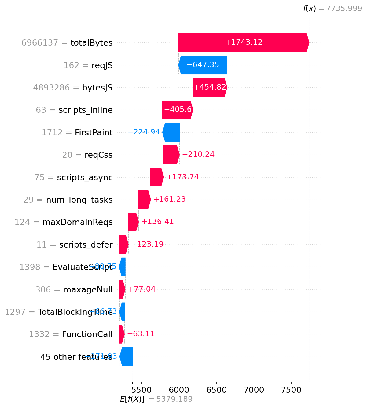
SHAP waterfalls
In addition to the text output, aislow.py generates a waterfall which is a visual representation of how we got from the baseline prediction to the final prediction for this specific page.
The plot starts with E[f(x)], the Expected value of f(x), which is the average SI prediction across all training data. This is the baseline meaning what we would predict if we knew nothing about the page.
Then each feature adds or subtracts from this baseline, shown as horizontal bars on the waterfall:
- Bars extending right (red/orange) are features making the page slower
- Bars extending left (blue) are features making it faster
The waterfall cascades from the baseline through the top ~15 most impactful features, ending at f(x) – the final prediction for this specific page.
Here’s the waterfall for the last run results you saw above:
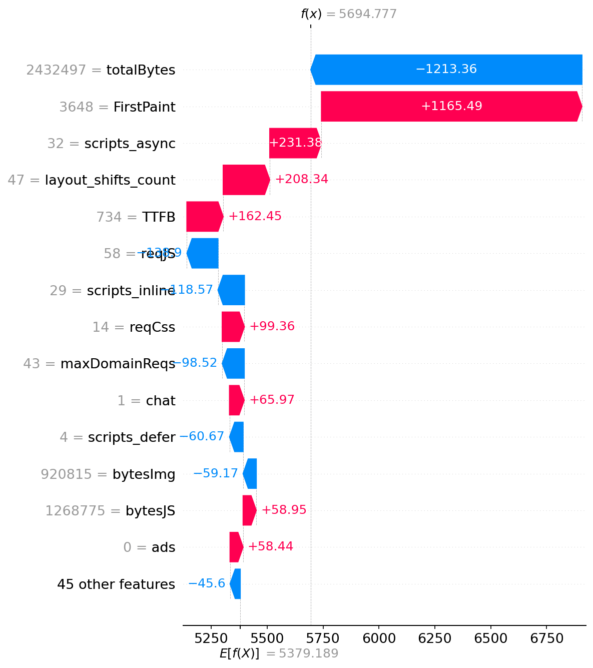
This waterfall helps visualize which features are the important contributors. In this case, First Paint dominates – that single metric adds over 1 second to the SI. Meanwhile, the relatively small page size saves over a second compared to the bloated average page in our dataset.
The text output and waterfall complement each other – the text gives you exact numbers and actionable advice, the waterfall gives you the big picture at a glance.
Here’s another example where things are going well reducing the predicted SI
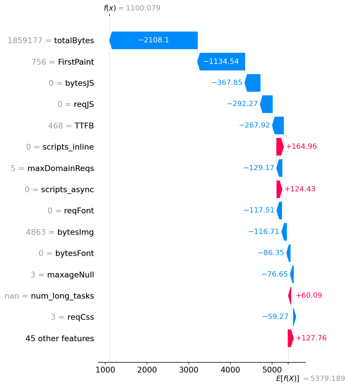
And here’s another example showing where things are mostly bad contributing to increased SI:
Parting words
So that’s aiSlow – YSlow reborn in the age of machine learning, trained on real-world data and attempting to tell us not just that a page is slow, but exactly why and by how much. And also what would be the top thing (or 5) to do to improve. And also telling us that if you fix the #1 top brokenness, how much can you expect to gain.
Obviously this humble aiSlow is not going to put any web perf consultant worth their salt out of business. But this is partially my fault, for training the model on incomplete (e.g. no response bodies) or irrelevant (e.g. caching headers) data when SpeedIndex is the goal. There could also be a false correlation on the part of the model. E.g. it may conclude based on the data that sites with GTM are faster, ergo using GTM is good. That’s patently false, it just so happens that sites who care enough to have a business that can use tracking, are also sites that may have better developers working on them. Another possible flaw in selecting relevant data (features) is selecting numbers that all measure or correlate to the same underlying cause. That’s why at some point I excluded a number of First(Contentful|Meaningful|Image)Paint metrics.
Clearly further tweaking is a TODO, this was just my first attempt. My hope is that it piqued your interest to try some ML on your own.
As a DIY-loving person, it irks me that we mostly consume models (via APIs or via chats) trained by the big players out there. The promise of AI (that I’d like to believe) is to democratize knowledge and access, right? It’d help if more of us are dipping into ML and not just sitting on the sidelines.
Disclaimer: most of the code is written by Cursor (Claude), I just tried to organize it better and hopefully ask the right questions to nudge towards a desired outcome.