Web Performance Calendar

I didn’t have anything planned for the Web Performance Calendar this year. That all changed after I read Tim Vereecke’s interesting proposal about a “Frustration Index” on Day 17.

His post got my attention, as a performance analyst, because some things looked familiar to me, while other things confused me. Eventually, it all became a bit frustrating. 🙂 As usual, that means I have to pull the whole thing apart and reconstruct it in my own way. So, this is a kind of a rushed mini-report about what I discovered. Among other things, perhaps it will also help you to better understand Tim’s approach. Accordingly, if you haven’t already, you should go and read his post because I will be drawing on that material quite heavily.

Frustration Over Indexes

Part of my confusion stemmed from having previously analyzed something called the Apdex Index (Application Index), which also defines a Frustration metric for web-page loading times. It also has metrics called, Tolerating and Satisfied. So, my first reaction was, nothing new. On a closer reading, however, it it became clear that the resemblance with Apdex is only superficial.

In a nutshell, the key observations motivating Tim’s Frustration Index (hereafter denoted “FI”) are:

• There are multiple performance tools available for measuring the times to render various components of a web page.
• Each tool has its own metric, e.g, Time To First Byte (TTFB), First Content Paint (FCP), and so on.
• This panoply of performance metrics raises an obvious question: Which one is best for optimizing web page performance?
• Taken on their own, none of them is ideal. Tim suggests taking the time differences between the various page load-time metrics. He calls this difference a “gap”; a term I found rather confusing.
• These differences, or gaps, are then used to calculate a single figure of merit he calls the “Frustration Index”.
• The bigger the FI value, the more frustrated a user is likely to become.
• The goal for the front-end developer then, is to attain the smallest FI across the panoply of metrics rather than simply tuning a particular page-loading metric.

To put all this in perspective, let’s look at an example of how the FI is intended to work.

Tim’s Page Tuning Example

For brevity and continuity, I’m going to recycle Tim’s example, starting with Fig. 1.

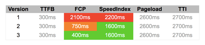
Fig. 1: Page component load-times (ms) from Tim’s post

I don’t know how realistic these times are but they are consistent and serve to illustrate both his points and mine. The rows in Fig. 1 correspond to three different versions of webpage code and therefore have different component load-times. The columns show the different performance-tool metrics along with their respective load-times measured in milliseconds (ms).

Tim presents these performance data more visually in Fig. 2, along with the associated FIs on the left side of the chart. The vertical order of the bars is the same as the order of the table rows. The point being illustrated is that reducing the time between the appearance of the Title and the Content in code Version 3 (FI = 15%), doesn’t produce the smallest FI because it has inadvertently increased the effective time between Content and Visually ready. It’s increased that gap relative to Version 2. Incidentally, the mismatch between the metric names in Fig. 1 and the labels in Fig. 2
was another source of confusion for me.

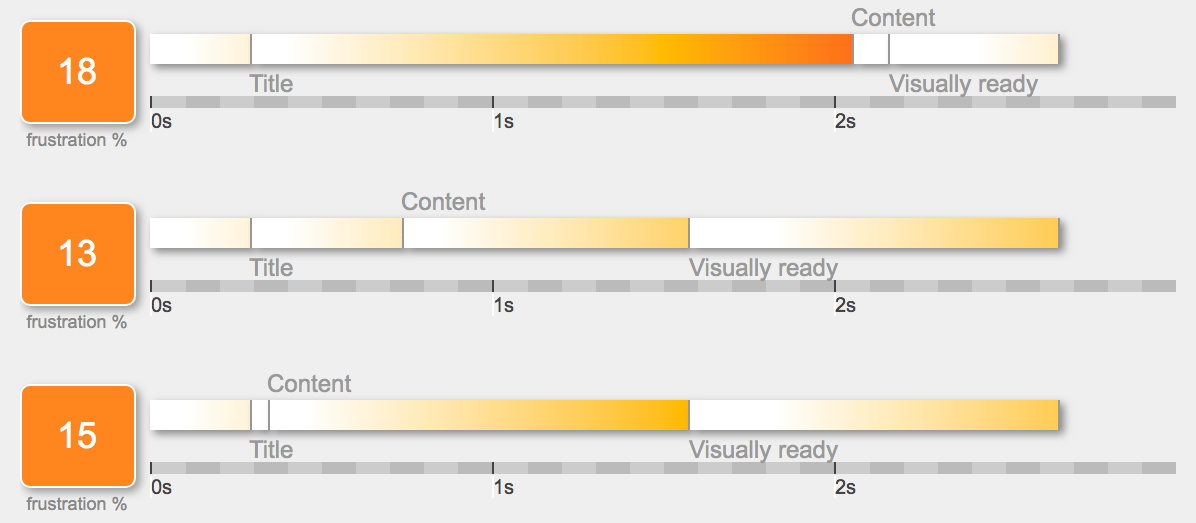
Fig. 2: Page component times with corresponding FIs from Tim’s post

Since Version 2 has the smallest FI, viz., 13%, it will have the best load performance, as perceived by a user. Moreover, note that the overall load time (TTI) has not changed in any of the versions. That is to say, none of the versions is loading any faster. What has happened in Version 2 is, the distribution of times to get the various components rendered, has improved. Hence, the user should feel less frustrated. At Xerox PARC, we used to call it “user pacification”.

Central Tenet:
This is the central tenet that motives the construction of the FI in the first place. Naively reducing the load-time based on one metric can result in the well-known hurry up and wait effect. It’s analogous to the impulse to speed up your CPU while leaving the I/O subsystem untouched. If the workload is I/O-bound, there won’t be much perceptible performance improvement. The FI is intended to help you avoid falling into that trap.

The FI is a very subtle metric because it borders on the psychology and psychophyics of user perception, which can be notoriously difficult to quantify unambiguously.

Closer Scrutiny

To understand where I’m coming from, I need to restate some aspects of Tim’s Example a little more rigorously.

1. The times in Fig. 1 are elapsed times. That’s the interval of time from when you start the stopwatch (or “timer”) until you stop it.
2. Those times are an ordered set: TTFB < FCP < … < TTI. In Fig. 1, each tool (and its metric) measures progressively longer rendering times for each page component. This is logically consistent since it would make no sense to have Speed < TTFB, for example. I will refer to this as the monotonicity condition.
3. It’s assumed that the total elapsed time to build the entire page (represented here by TTI) remains invariant in the tuning process (i.e., between versions). In practice, your mileage may vary but, for the purposes of illustration, this is a perfectly reasonable simplifying assumption.
4. From a mathematical standpoint, the timing metrics are ranked data.
5. The gap refers to the difference between successive pairs of metrics in the ranked data.
6. Mathematically speaking, a “gap” is just the delta time:
   Δt = t2 - t1,
   where t₁ < t₂ are any pair of successive elapsed times. It’s the interval of time from the end of one page-timer to the end of its successor page-timer, i.e., the difference between two timer intervals. We already have a name for that in performance analysis.
7. Modulo ± signs, it’s precisely these Δt’s that are used in the PHP function calculateFrustrationPoints() as part of computing the FI value. (See Tim’s code box)
8. It’s assumed that Δt ≥ 100, i.e., the minimal measurable difference between each page metric is 100 ms. He refers to it as a threshold. I’ll retain this assumption. Actually, there’s a certain amount of monkey business in the PHP code regarding how these thresholds are used to calculate the Δt’s, e.g., one threshold = 250, not 100. I’m going to ignore that level of detail in what follows.
9. The FI values, computed by the PHP function calculateFrustrationIndex() (see his code box), are actually real numbers, not integers. In Fig. 2, however, they’ve been rounded up to the nearest integer value (no decimal). As we’ll see shortly, this rounding can hide information so, I won’t employ it.

With those qualifications in place, I’m now going to take a different slant on the FI concept.

Let’s Get Vertical

The first thing I want to do is display the elapsed times as vertical bars with the Version FI shown above them. In other words, Fig. 3 corresponds to Fig. 2 but with each of the elapsed times represented by separate side-by-side vertical bars that are ordered by increasing height, as prescribed by the monotonicity condition listed earlier. Also, from here on, I’ll use decimal values of the FI, without any rounding.

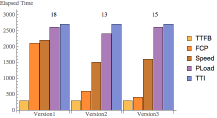
Fig. 3: Elapsed page-component times with their respective rounded FIs (cf. Fig. 2)

Next, I want to introduce a new element. Fig. 4 shows the same data as Fig. 3 but with the addition of a diagonal line or diagonal gradient superimposed on each group of columns belonging to the respective version of the page-code.

Fig. 4: Elapsed times with diagonal gradients

I would now like to make the following observations concerning Fig. 4:

1. All the diagonal gradients have the same slope. Reading left to right, each diagonal begins at the center-top of the lowest column (the TTFB elapsed time) and terminates at the center-top of the highest column (the TTI elapsed time). Since the TTFB and TTI metrics have the same values in each Version, the diagonal lines all slant at the same angle.
2. Version 2, which has the lowest FI value (12.74), happens to have all its columns closest the diagonal gradient.
3. In Version 1, on the other hand, the three central columns are higher than the diagonal gradient and its FI value (17.30) is also higher than Version 2.
4. In Version 3, the second column is significantly lower than the diagonal, while its fourth column is higher than the diagonal. Accordingly, its FI value (14.04) is also higher than Version 2.

From these observations, I draw the following hypothesis. Column heights (elapsed times) that lie nearest to the diagonal gradient have the lowest FI value. Any departure from the diagonal gradient (up or down) increases the FI value. In other words, the diagonal gradient is some kind of a minimization criterion.

Fig. 5: Elapsed times for Versions 1, 2 and 3 compared with Optimal times

In Tim’s Page Tuning Example, we saw that the FI value was lowest for Version 2 code. Now, we also see that that FI value wasn’t the lowest possible FI value.

Even without fully understanding what’s going on here, it already suggests an alternative performance objective for a front-end developer.

Developer Goal:
Optimal performance will be attained by tuning the application code so that the ranked page metrics fall on the diagonal gradient defined between TTFB and TTI for that application.

To pull this off, you need to know how to generate the diagonal gradient. Not a big deal. From high school you will recall that the general equation for a straight line is given by y = m x + c, where m is the slope of the line and c its y-axis intercept. Here, since monotonicity guarantees the same ordering of the page-loading metrics, we can simply index them as x = 1, 2, ..., 5. Then, the m and c values can be calculated as:

m = (TTI - TTFB) / 4
c = TTFB - m

Thus, the diagonal lines in Fig. 5, where TTFB = 300 ms and TTI = 2700 ms, correspond to m = 600 and c = −300.

Using this diagonal gradient, the previous loading times in Fig. 1 can now be compared numerically with the optimal time shown in Fig. 6. Unlike Version 2 tuning, we now see that optimal performance is achieved by making the FCP time longer than Version 2 by 300 ms, while the PLoad time has been reduced simultaneously by 300 ms.

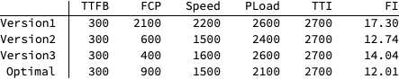
Fig. 6: Comparison of diagonal-gradient optimal times with elapsed times in Fig. 1

Fig. 6 offers some strong evidence that there’s a relationship between the diagonal gradient and the FI. On the other hand, this is a small measurement sample and maybe we just got lucky with these particular loading times. It would be more convincing if we could find a formal connection.

Euclidean Norm

In Tim’s PHP code the equivalent of the Δt’s (i.e., the difference in elapsed times) are labelled A, B, C, D and it will now be convenient to use that notation to understand the connection between the FI and th diagonal gradient. Since A, B, C, D are independent variables (after all, they’re usually measured independently by different tools) they can be represented mathematically on separate axes in a Cartesian coordinate system where each of the axes are orthogonal to one another: also known as basis vectors.

For the data in Fig. 1, however, we need four axes for A, B, C, and D, and there’s no convenient way to visualize that. So, without loss of generality, I’m going to restrict myself to 3-dimensions just for ease of visualization. Moreover, I’m going to consider the simplest possible case where A = B = C = 100 ms (the required “threshold” that Tim invokes). That corresponds to an absolute minimum gradient with a small Frustration Index value, e.g., FI = 2 (depending on how you count). Not particularly realistic but, much it makes the math easier to understand.

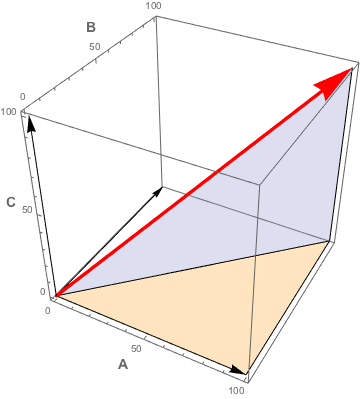
Fig. 7: Minimum FI basis vectors (black) and the resultant vector (red)

Fig. 7 highlights the basis vectors A, B, and C as black arrows eminating from the lower left corner. The length of big red arrow, it turns out, corresponds to the FI metric. To find its length we can use the famous theorem of Pythagoras but, in 3-dimensions. Luckily, this is just a matter of applying the familiar 2-dimensional theorem to the correct sequence of right-triangles. Recall the 2-dimensional version of Pythagoras states that the square of the hypotenuse is equal to the sum of the squares on the other two sides.

It’s clear in Fig. 7 that the length of the red arrow corresponds to the hypotenuse (H) of the vertical blue right-triangle, and the base of that blue triangle corresponds to the hypotenuse of the horizontal yellow right-triangle, and so on. You get the idea. Algebraically, this simplifies to

  H2 = A2 + B2 + C2

In other words, H can be calculated directly from the basis vectors A, B, and C as the sum of squares.

Sum of squares is the reason that the pow(..., 2) function makes an appearance in Tim’s code box.

In this simple case, H² = 100² + 100² + 100² = 30,000. Taking the square root, (and dividing by 100 to be consistent with Tim’s FI code), we find H = 1.73.

The generalization of H, to 4 (or more dimensions), is called the Euclidean norm:

Norm = √ ( A² + B² + C² + D² )

If we repeat the same procedure algebraically in 4-dimensions with A = B = C = D = 100 ms (not easy to visualize), we find Norm = 2, as promised. This is essentially the same result you would get by using the PHP code to calculate the FI with a set of elapsed times that differ by 100 ms, e.g., (300, 400, 500, 600, 700) has an FI = 2.06155. The difference comes from the way the basis vectors are scaled in the PHP code.

Actual page-load deltas, A, B, C, and D, will usually be very different from one other (cf. Fig. 1). That means the red arrow in Fig. 6 can have any unbounded length (and it can point in different directions). For the Version 1 elapsed times, Tim’s PHP code produces A = 200, B = 1700, C = 0, and D = 250. Substituting these values into the Norm equation above (and dividing by 100), we find Norm = 12.73 in agreement with Fig. 6.

Shortest Path

So far, I’ve demonstrated that the numerical value of FI is the same as the Euclidean norm in a 4-dimensional metric space defined by the basis vectors A, B, C, and D. That’s essentially what Tim’s PHP code box computes. Now, I would like to understand how the Euclidean norm computation is related to the diagonal gradient minimization observed in Figs. 4 and 5.

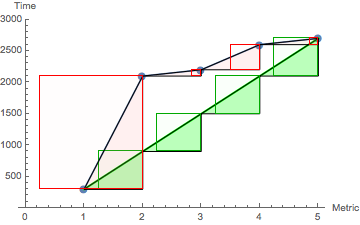
Fig. 8: Version 1 path lengths together with associated triangles and squares

The diagonal gradients in Fig. 5 are all identical because they correspond to the distance between the same end points defined by TTFB and TTI (the end columns in Fig. 5). The geometrical significance of the diagonal gradient is made more explicit in Fig. 8. That diagram focuses on Version 1 elapsed times, with the vertical columns now replaced by dots. Additionally, these dots are joined by short line segments. The upshot is to produce a piecewise linear curve between the end points TTFB and TTI.

The corresponding diagonal gradient for Version 1 is shown in green. Looked at as curves, it’s clear that the upper curve is longer than the diagonal path. If the upper curve was elastic and sitting on blue “pegs” then, optimizing Version 1 elapsed times would be analogous to reducing the elastic tension by moving the pegs downward until they all lay on the diagonal: the shortest Euclidean distance between TTFB and TTI.

Moreover, the delta times (analogous to A, B, C, and D) are shown as heights of the pink triangles. If we also extend those heights in the horizontal direction, we obtain the analogous squares of A, B, C, and D, which are precisely the terms used to compute the previous Norm equation, i.e., the FI. Conversely, the green triangles belonging to the diagonal gradient are all identical in height. As a consequence, the associated squares are also identical. When we sum the areas of the green squares, we get a smaller total area than for the pink squares.

The green triangles with identical heights are logically equivalent to the basis vectors of the previous section. Similarly, the identical green squares define the optimal Euclidean norm.

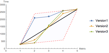
Fig. 9: Bounding parallelogram of paths corresponding to Fig. 1

Finally, because of the monotonicity condition on the elapsed times, there are bounds on the data. That boundary is a parallelogram whose size is determined by the values of TTFB and TTI. Curves (i.e., elapsed-time data) like the one in Fig. 8 can only exist inside this parallelogram. To make this more apparent, Fig. 9 gathers the data from Versions 1, 2 and 3 into this bounded area.

Summary

This post has primarily presented two things.

1. That the Frustration index is the Euclidean norm in the vector space of component page-load metrics. This concept is already contained in in Tim’s PHP code. I’ve merely explained how it works. Strictly speaking, since the norm can be unbounded, the FI is not really a percentage (as denoted in Fig. 2). For example, if the TTI had a value like 50,000 ms, the FI = 301.498. In practice, however a load time like that is more likely to be regarded as an abuse of the word performance. These days, a TTI greater than 5,000 ms is already likely to be considered unacceptable. Nonetheless, once the normalizations are fixed, the FI values can be compared to one another.
2. The elapsed times can also be identified with piecewise linear curves bounded by the end points TTFB and TTI. The path-length of such curves will usually be greater than the corresponding diagonal gradient between the same end points: the shortest path. The bounding parallelogram of these curves captures the monotonicity constraint on the page-load data. The performance goal for the front-end developer can therefore be expressed as minimizing the path length by reducing the elapsed-time components until the curve becomes the shortest path that belongs to the diagonal gradient. I explained how you can easily calculate the the slope and intercept of the diagonal gradient. The diagonal gradient guarantees the Δt’s or gaps are optimized, and also ensures the FI will be the smallest.

Both of these approaches can be regarded as variants of a quadratic minimization procedure.

Although the FI is not absolutely necessary to improve performance, it’s available as an option when accurate numerical (non-integer) comparisons are needed. Similarly, I could come up with an alternative figure of merit based instead on quadratic minimization of the diagonal gradient that would have a guaranteed range between 0% and 100%. But, that’s possibly a topic for Web Performance Calendar 2020.